- Tworzymy nowy projekt i ustawiamy zmienne środowiska.
import findspark
findspark.init()
from graphframes import *
from pyspark.sql.types import *
from pyspark.sql import functions as F
import matplotlib
import matplotlib.pyplot as plt
plt.style.use('fivethirtyeight')
from pyspark.sql import SparkSession
spark = SparkSession.builder.appName('baza').getOrCreate()
- Wczytanie wartości opisy portów lotniczych - węzły.
nodes = spark.read.csv("/home/spark/lab04/task4/airports.csv", header=False)
nodes.columns
cleaned_nodes = (nodes.select("_c1", "_c3", "_c4", "_c6", "_c7")
                 .filter("_c3 = 'United States'")
                 .withColumnRenamed("_c1", "name")
                 .withColumnRenamed("_c4", "id")
                 .withColumnRenamed("_c6", "latitude")
                 .withColumnRenamed("_c7", "longitude")
                 .drop("_c3"))
cleaned_nodes = cleaned_nodes[cleaned_nodes["id"] != "\\N"]
- Wczytanie wartości relacji - krawędzie.
relationships = spark.read.csv("/home/spark/lab04/task4/188591317_T_ONTIME.csv", header=True)
cleaned_relationships = (relationships
                         .select("ORIGIN", "DEST", "FL_DATE", "DEP_DELAY", "ARR_DELAY",
                                 "DISTANCE", "TAIL_NUM", "FL_NUM", "CRS_DEP_TIME",
                                 "CRS_ARR_TIME", "UNIQUE_CARRIER")
                         .withColumnRenamed("ORIGIN", "src")
                         .withColumnRenamed("DEST", "dst")
                         .withColumnRenamed("DEP_DELAY", "deptDelay")
                         .withColumnRenamed("ARR_DELAY", "arrDelay")
                         .withColumnRenamed("TAIL_NUM", "tailNumber")
                         .withColumnRenamed("FL_NUM", "flightNumber")
                         .withColumnRenamed("FL_DATE", "date")
                         .withColumnRenamed("CRS_DEP_TIME", "time")
                         .withColumnRenamed("CRS_ARR_TIME", "arrivalTime")
                         .withColumnRenamed("DISTANCE", "distance")
                         .withColumnRenamed("UNIQUE_CARRIER", "airline")
                         .withColumn("deptDelay", F.col("deptDelay").cast(FloatType()))
                         .withColumn("arrDelay", F.col("arrDelay").cast(FloatType()))
                         .withColumn("time", F.col("time").cast(IntegerType()))
                         .withColumn("arrivalTime", F.col("arrivalTime").cast(IntegerType()))
                         )
- Utworzenie struktury GraphFrame.
g = GraphFrame(cleaned_nodes, cleaned_relationships)
- Odczyt z pliku referencji kodów do nazw linii lotniczych.
airlines_reference = (spark.read.csv("/home/spark/lab04/task4/airlines.csv")
      .select("_c1", "_c3")
      .withColumnRenamed("_c1", "name")
      .withColumnRenamed("_c3", "code"))
airlines_reference = airlines_reference[airlines_reference["code"] != "null"]
df = spark.read.option("multiline", "true").json("/home/spark/lab04/task4/airlines.json")
dummyDf = spark.createDataFrame([("test", "test")], ["code", "name"])
for code in df.schema.fieldNames():
    tempDf = (df.withColumn("code", F.lit(code))
              .withColumn("name", df[code]))
    tdf = tempDf.select("code", "name")
    dummyDf = dummyDf.union(tdf)
- Troszkę statystyki, liczba węzłów, krawędzi i maksymalny czas opóźnienia.
g.vertices.count()
g.edges.count()
g.edges.groupBy().max("deptDelay").show()
- Szukamy lotnisk z których odlatuje najwięcej samolotów. Wykorzystamy algorytm oparty o "Degree Centrality".
airports_degree = g.outDegrees.withColumnRenamed("id", "oId")
full_airports_degree = (airports_degree
                        .join(g.vertices, airports_degree.oId == g.vertices.id)
                        .sort("outDegree", ascending=False)
                        .select("id", "name", "outDegree"))
full_airports_degree.show(n=10, truncate=False)
- Prezentacja graficzna najbardziej popularnych lotnisk ( w oparciu o stopień węzłów ).
plt.style.use('fivethirtyeight')

ax = (full_airports_degree
      .toPandas()
      .head(10)
      .plot(kind='bar', x='id', y='outDegree', legend=None))

ax.xaxis.set_label_text("")
plt.xticks(rotation=45)
plt.tight_layout()
plt.show()
- Kolejna analiza przedstawia zestawienie opóźnień lotów z lotniska ORD (Chicago O’Hare International Airport),
ważny węzeł komunikacyjny pomiedzy wschodnim i zachodnim wybrzeżem. Prezentacja 10 najbardziej opóźnionych lotów.
delayed_flights = (g.edges
                   .filter("src = 'ORD' and deptDelay > 0")
                   .groupBy("dst")
                   .agg(F.avg("deptDelay"), F.count("deptDelay"))
                   .withColumn("averageDelay", F.round(F.col("avg(deptDelay)"), 2))
                   .withColumn("numberOfDelays", F.col("count(deptDelay)")))
(delayed_flights
 .join(g.vertices, delayed_flights.dst == g.vertices.id)
 .sort(F.desc("averageDelay"))
 .select("dst", "name", "averageDelay", "numberOfDelays")
 .show(n=10, truncate=False))
- Na pierwszym miejscu jest 12 lotów z lotniska ORD do lotniska CKB. Przeprowadzamy
dalszą analizę tych lotów.
from_expr = 'id = "ORD"'
to_expr = 'id = "CKB"'
ord_to_ckb = g.bfs(from_expr, to_expr)
ord_to_ckb = ord_to_ckb.select(
  F.col("e0.date"),
  F.col("e0.time"),
  F.col("e0.flightNumber"),
  F.col("e0.deptDelay"))
ax = (ord_to_ckb
      .sort("date")
      .toPandas()
      .plot(kind='bar', x='date', y='deptDelay', legend=None))

ax.xaxis.set_label_text("")
plt.tight_layout()
plt.show()
- Analiza wykresu. Ponad połowa lotów była opóźniona. Ale największe opóżnienie było
2 maja 2018 i wynosiło 14 godzin co wpłynęlo na niekorzystny wynik.
- Analiza lotów na lotnisku San Francisco International Airport (SFO) w dniu 11-05-2018 - zły dzień.
( Analizujemy dzień w którym najwięcej było opóźnień na lotnisku ).
W ramach tego punktu znajdziemy lotu które lądują na lotnisku a następnie odlatują - (a)-[ab]->(b); (b)-[bc]->(c).
Znajdujemy loty, które mają opóźnienie przylotu lub odlotu powyżej 30 minut i należą do tej samej linii.
motifs = (g.find("(a)-[ab]->(b); (b)-[bc]->(c)")
          .filter("""(b.id = 'SFO') and
                  (ab.date = '2018-05-11' and bc.date = '2018-05-11') and
                  (ab.arrDelay > 30 or bc.deptDelay > 30) and
                  (ab.flightNumber = bc.flightNumber) and
                  (ab.airline = bc.airline) and
                  (ab.time < bc.time)"""))
def sum_dist(dist1, dist2):
    return sum([value for value in [dist1, dist2] if value is not None])
sum_dist_udf = F.udf(sum_dist, FloatType())
result = (motifs.withColumn("delta", motifs.bc.deptDelay - motifs.ab.arrDelay)
          .select("ab", "bc", "delta")
          .sort("delta", ascending=False))
result.select(
    F.col("ab.src").alias("a1"),
    F.col("ab.time").alias("a1DeptTime"),
    F.col("ab.arrDelay"),
    F.col("ab.dst").alias("a2"),
    F.col("bc.time").alias("a2DeptTime"),
    F.col("bc.deptDelay"),
    F.col("bc.dst").alias("a3"),
    F.col("ab.airline"),
    F.col("ab.flightNumber"),
    F.col("delta")
).show()
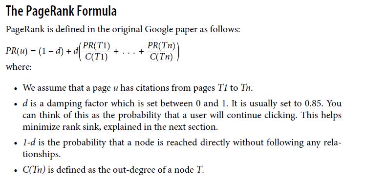
- Wyznaczenie wartości Page Rank (obliczenia troszkę trwają, można pominać, wrócić później).
result = g.pageRank(resetProbability=0.15, maxIter=20)
(result.vertices
 .sort("pagerank", ascending=False)
 .withColumn("pagerank", F.round(F.col("pagerank"), 2))
 .show(truncate=False, n=100))
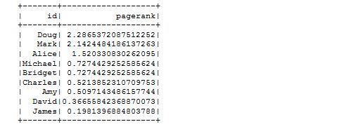
- Wyznaczenie wartości Page Rank (obliczenia troszkę trwają, można pominać, wrócić później).
triangles = g.triangleCount().cache()
pagerank = g.pageRank(resetProbability=0.15, maxIter=20).cache()

(triangles.select(F.col("id").alias("tId"), "count")
 .join(pagerank.vertices, F.col("tId") == F.col("id"))
 .select("id", "name", "pagerank", "count")
 .sort("count", ascending=False)
 .withColumn("pagerank", F.round(F.col("pagerank"), 2))
 .show(truncate=False))
- W kolejnym zadaniu poszukimy linii lotniczej, która umożliwi nam zwiedzenie największej liczby lotnisk.
airlines = (g.edges
  .groupBy("airline")
  .agg(F.count("airline").alias("flights"))
  .sort("flights", ascending=False))
full_name_airlines = (airlines_reference
  .join(airlines, airlines.airline == airlines_reference.code)
  .select("code", "name", "flights"))
ax = (full_name_airlines.toPandas()
  .plot(kind='bar', x='name', y='flights', legend=None))
ax.xaxis.set_label_text("")
plt.tight_layout()
plt.show()
- Kolejny algorytm pozwoli nam znaleźć grupy lotnisk dla każdej linii lotniczej,
których loty z i do lotnisk należą do tej samej grupy. Wykorzystujemy algorytm
"Strongly Connected Components". ( Liczy długo )
Najwieksza liczba obsługiwanych lotnisk - linia loticza.
def find_scc_components(g, airline):
   # Create a subgraph containing only flights on the provided airline
   airline_relationships = g.edges[g.edges.airline == airline]
   airline_graph = GraphFrame(g.vertices, airline_relationships)
   # Calculate the Strongly Connected Components
   scc = airline_graph.stronglyConnectedComponents(maxIter=10)
   # Find the size of the biggest component and return that
   return (scc
     .groupBy("component")
     .agg(F.count("id").alias("size"))
     .sort("size", ascending=False)
     .take(1)[0]["size"])
# Calculate the largest strongly connected component for each airline
airline_scc = [(airline, find_scc_components(g, airline))
for airline in airlines.toPandas()["airline"].tolist()]
airline_scc_df = spark.createDataFrame(airline_scc, ['id', 'sccCount'])
# Join the SCC DataFrame with the airlines DataFrame so that we can show
# the number of flights an airline has alongside the number of
# airports reachable in its biggest component
airline_reach = (airline_scc_df
.join(full_name_airlines, full_name_airlines.code == airline_scc_df.id)
.select("code", "name", "flights", "sccCount")
.sort("sccCount", ascending=False))
- Prezentacja wyników na wykresie.
ax = (airline_reach.toPandas()
.plot(kind='bar', x='name', y='sccCount', legend=None))
ax.xaxis.set_label_text("")
plt.tight_layout()
plt.show()
- Podczas kolejnej analizy poznamy lotniska, które są obslugiwane przez przewoźnika DL ( Delta Airlines).
airline_relationships = g.edges.filter("airline = 'DL'")
airline_graph = GraphFrame(g.vertices, airline_relationships)

clusters = airline_graph.labelPropagation(maxIter=10)
(clusters
 .sort("label")
 .groupby("label")
 .agg(F.collect_list("id").alias("airports"),
      F.count("id").alias("count"))
 .sort("count", ascending=False)
 .show(truncate=70, n=10))
all_flights = g.degrees.withColumnRenamed("id", "aId")
(clusters
.filter("label=1606317768706")
.join(all_flights, all_flights.aId == clusters.id)
 .sort("degree", ascending=False)
.select("id", "name", "degree")
.show(truncate=False))